A Brief Look at Understanding the Limitations of MTBF

Mean-Time-Between-Failure (MTBF) as defined by the MIL-STD-721C Definition of Terms for Reliability and Maintainability (12 June 1981) is

[a] basic measure of reliability for repairable items: The mean number of life units during which all parts of >the item perform within their specified limits, during a particular measurement interval under stated >conditions.

MTBF is widely used to describe the reliability of a component or system. It is also often misunderstood and used incorrectly. In some sense, the very name “mean time between failures” contributes to this misunderstanding. The objective of this paper is to explore the misunderstood nature of MTBF and its impact on decision making and program costs.

Mean-Time-To-Failure versus MTBF

Related to MTBF is the Mean-Time-To-Failure (MTTF), defined as

[a] basic measure of reliability for non-repairable items: The total number of life units of an item divided >by the total number of failures within that population, during a particular measurement interval under stated >conditions.

The definitions of MTTF and MTBF are very similar. The subtle difference is important, yet the confusion is further complicated when one attempts to quantify MTBF or MTTF. In both cases we use the calculation as described within the MTTF definition. This is what we would do for any group of values that we wanted to find the mean (average) value estimate. Tally the values and divide by the number of hours all units have operated and divide by the number of failures. This provided a (statistically) unbiased estimate of the population mean.

Estimating MTTF or MTBF

Keep in mind that time-to-failure data are not normally distributed. The underlying distribution for life data starts at time zero and increases. The exponential family of distributions tends to describe life data well and is commonly used. The unbiased estimate for the mean value of an exponential distribution is as described for the MTTF definition above.

When working with data from a repairable system, one should use the nonhomogeneous Poison process, which is a generalization of the Poison distribution. Estimates for the failure intensity can be made from various models, yet often an exponential model is assumed. This results in the common estimate of

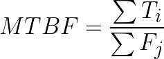
where T_{i<\sub> as the total time of system I divided by the cumulative number of failures, fj<\sub>. [1]}

MTBF and MTTF are easy to calculate. One can plot the data and compare them to the exponential distribution. If the data do not fit the distribution, then the assumption that MTBF applies is incorrect.

Calculating Reliability

The first source of confusion when considering MTBF has to do with choosing the appropriate distribution. Because we intuitively use a simple calculation to estimate the mean value, many then do not then apply that estimate with the reliability function of the appropriate distribution.

For example, if a vendor states that the product has an MTBF of 16,000 hours, and we wanted to know how many out of 100 units will fail in 8,000 hours, the appropriate calculation is to use the reliability equation

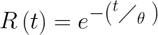
where t is time and θ is the desired MTBF. Then for our example

Thus we would expect 61 out of the 100 units, or 61%, of the units to operate for the full 8,000 hours.

In this calculation we have assumed an exponential distribution and nonrepairable units. Given only an MTBF value, the most likely distribution to use without additional information is the exponential.

Extending this same example to determine the reliability at 16,000 hours, we find that only about 1/3 of the units would be expected to still be operating. Having this common misunderstanding of the failure rate value that MTBF represents can lead to significant loss of resources or mission readiness.

MTBF is not

• a failure-free period,
• the 50th percentile of time-to-failure times,
• suitable for decreasing failure rates (early life failures), or
• suitable for increasing failure rates (wear out failures).

Rather, MTBF is

• the 63rd percentile of time-to-failure times,
• easy to calculate, and
• suitable for constant-failure-rate failure mechanisms (which rarely
  exist).