Samples for Testing

Normally, we life test a sample of products in order to make sure the products will last as long as expected. We assume that the sample we select will represent the total population of products that we eventually ship. It is not a perfect system, and there is some risk involved.
For example, the risk the sample doesn’t represent the population, or that the process for making the product changes and alters the final reliability. Or, the testing doesn’t reflect the use conditions and over or under estimates the resulting product reliability. Or, the test isn’t designed well.
A bad way to start planning a test is to begin with a MTBF and wish to demonstrate the product meets or exceeds that MTBF value.
The Sample Size for MTBF Demonstration
Lets say we have a product and we want to demonstrate it has a 5 hour MTBF. And, let’s say we have five samples available for testing. If we test the products for 25 hours, that is a total of 5 x 25 = 125 hours of testing. We count the number of failures (fix and return the product to testing) and if we get 25 or fewer failures, we can calculate the MTBF estimate based on the data, as 125 hours / 25 failures = 5 hours MTBF. Pretty simple.
A common way to estimate the sample size needed to show a particular MTBF with a particular sampling confidence is done with the Χ2 distribution and the following formula.
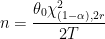
θ is our desired MTBF to demonstrate. X2 is the chi-squared distribution with degrees of freedom determined by α which is related to the Type I confidence, and r, which is the critical number of failures. T is the total hours of operation across all units in the test. Working with this formula is left as an exercise for those interested.
We can design the test based on the constraints we have, such as sample size or test duration. A little algebra permits solving with either constraint.
Constant Failure Rate Assumption Issue
The assumption made when using this approach is that the failure rate is constant. The chance to fail is the same at hour one and hour 100. This permits the accumulation of operating hours across various machines to tally the total hours.
If the test is designed to tally 200 hours, one unit could run 199 hours and the other 1 resulting in a T = 200 hours. That’s ok. Or we could have 200 units each operate one hour. Or, one unit run the entire time. As long as some number of units run for T time in total, this approach is fine.
It is this ‘feature’ that first caused me to look at this approach a bit more closely. While it if fine when the assumption is valid, it will produce meaningless results if the constant failure rate is not valid. While we all feel more confident when a reliability figure is supported by test data, it is generally not comforting when one realizes what it really means. Nothing.
It is common to see MTBF values reported without a corresponding duration over which it is valid. That confused look you see when asking for a duration along with an MTBF values is a topic for another post. Yet, the idea that the MTBF value (the constant failure rate) is valid indefinitely is laughable.
It is possible to support with test data nearly any MTBF value. For example, component suppliers often run short duration testing on many units. Over time that accumulated test time, T, becomes quite large and the number of failures is often zero or very, very low. Thus, they can support a very high MTBF value – which is meaningless beyond the operating time units experience during testing.
How do you determine sample size for life testing? If it starts with the notion of demonstrating an MTBF value, you may need to reevaluate your approach.
Fred,
That chi-squared formula you used also relies on having so many failures that the CLT can apply. Most of our products these days have such high reliability requirements that we won’t get enough data for the CLT to be valid.
Mark Powell
Hi Mark,
Had not thought about central limit theorem. It’s still a bad approach though.
cheers,
Fred
Asking the suppliers that only supply MTBF information as to how their testing was complete and how many samples were used to caculate. We never take just MTBF as the final approval.
An important consideration is that you only demonstrate the reliability (not failure rate, MTBF, or even hazard rate) at the time applicable to the end of the test–unless you also know the distribution of the data.
A better way is to use some of the methods of life data analysis. Even with a limited number of failures, you can get an idea of the shape of the low percentiles (a fair amount of my data is lognormal). You can (with some risk) extrapolate to percentiles of interest.
It’s also worth mentioning that a fair amount of this sort of testing is actually done under elevated stresses. That is a path that must be trodden with caution. Beware when a failure mode shows up at say 100C that doesn’t show up at 80C.
Hi Paul,
Good comment and I agree. Focus on the goal, a reliable product, and measure that with your testing and modeling/estimate. Totally agree.
Hard part is who to do and what testing to do – as you mention accelerated testing is not always obvious or easy. Multiple failure mechanisms, accelerating stresses, etc. can all make this a lot of ‘fun’. It’s what keep our role interesting.
Cheers,
Fred