Give me a place to stand on, and I will move the Earth.
Archimedes
Its known HALT is an effective way to find the weaknesses in your product during the reliability improvement program. In doing so, we view HALT as a qualitative test only. We cannot define the reliability and lifetime of the product from its results. So, unfortunately, we cannot use HALT for purposes of Type Certification, confirm the lifetime of Critical Parts, predict the warranty and maintenance costs, which are required, for example, for aviation.
If we could combine the effectiveness of HALT (high acceleration of testing) with the benefits of quantitative testing, we would get a very powerful tool for the Reliability Demonstration and the Reliability Development of the new products.
Let us consider in detail why the HALT has not become a quantitative test so far and whether it can become one.
We can get quantitative characteristics of reliability and lifetime by two methods. This is a MEASUREMENT and EVALUATION (See Part 1).
HALT failure data is clearly not enough for the MEASUREMENT of reliability and lifetime due to the small numbers of samples and failures.
Therefore, we can get quantitative characteristics only by the EVALUATION method.
And EVALUATION of reliability and lifetime is impossible due to a lack of mathematical foundation, besides expressions like 1-CL=Rn with its inherent disadvantages (See Part 2) and software tools, besides Reliasoft’s Weibull++ DRT utility. This impasse is the reason that the HALT remains qualitative.
The way out of this impasse is the creation of a new mathematical foundation by explicit consideration of uncertainty and its resolution by the worst-case method (Part 3). “Give me a place to stand on, and I will move the Earth” (Archimedes). THIS IS THE PLACE! We do not know something. Let us make evaluations and build the best control based on the worst-case scenario.
There are simple formulas (Part 3). Unfortunately, this is where the simplicity ends:
1. We must consider all possible events (often dependent) during testing and operation of the product and calculate their probabilities. As Kozma Prutkov used to say, “You can’t grasp the immensity!”
2. What is the indicator of the worst case? For some, it is a risk, for another it is safety. A more general indicator of the worst case can be the Life Cycle Cost of the product.
This approach is implemented in the software tool Life Cycle Simulator, which calculates the quantitative characteristics of reliability and lifetime from HALT data.
Even more interesting tasks that the Simulator solves are:
– Finding the best-accelerated testing modes that will provide the smallest Life Cycle Cost for a given Time to Market.
– Search and foundation for absolutely new test acceleration methods.
We can make a simple example to demonstrate this approach. This example is so simple that we can do calculations in Excel.
We are making a Reliability Improving Program of the product. The expected product launch program is 50 units. The warranty lifetime is 6000 hours. The warranty costs are $20 per failure.
The product has one failure mode with a normal distribution of lifetime. The lifetime expectation is unknown, but it is in the range of 3000 – 13000 hours. The standard deviation is 900 hours.
The Reliability Improvement Program of the Product includes the testing of one product. The cost of the product for testing is $15. The cost of the testing gas-hour is $0.01.
If a product passes the test, it goes into production. The production cost of the basic version is $10 per product. If the product fails the test, we redesign the product. The cost of the redesign is $10. The production cost of the redesigned version is $12 per product. We suppose the modified product does not fail for warranty lifetime
Applying this approach, we review the uncertainty of the lifetime expectation (from 3000 to 13000 hours). Let the duration of our test will be 6,000 hours for example. Then we will have probabilities of passing the test as shown in Line 1 of Table 1.
The expectation of the Development cost (including the cost of the product to test, the cost of the test itself, and the cost of the redesign, if necessary) calculated for the discrete distribution is shown in Line 2 of Table 1.
The expectation of the Manufacture cost (considering the production of basic or modified versions) calculated for the discrete distribution is shown in Line 3 of Table 1.
The expectation of the Warranty cost calculated by Poisson distribution is shown in Line 4 of Table 1.

The total cost of the product life cycle is shown in Line 5 of Table 1.
Brief explanation: as the life of the product increases, the probability of passing the test increases from 0 to 1. The expectation of the development cost decreases from $85 to $75 due to the decrease in the probability of redesign. The expected manufacturing cost is reduced from $600 to $500 due to the reduced probability of producing a more expensive redesigned version. The expected warranty cost first rises from 0 to $250 and then decreases to 0. This is due to the fact that a bad product will be identified in testing and redesigned, and warranty costs will be minimal. A good product will have minimal warranty costs too. The middle of uncertainty is the worst! The life cycle cost of the product is a maximum of $880 with an expected lifetime of 6000 hours.
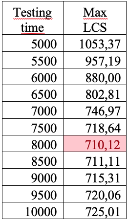
We solved the problem of uncertainty by looking for the worst case. Now we can find the best control (test time) at which the life cycle cost is minimal (See Table 2). This is $710 with a test time of 8000 hours.

We can also find the best control (the number of samples for testing) at which the life cycle cost is minimal. In this case, an increase in the number of tested samples from 1 to 2 and 3 increases the expected life cycle cost from 710 to 787 and 859, which are not beneficial. If we don’t test, the expected life cycle cost will be $ 1500.
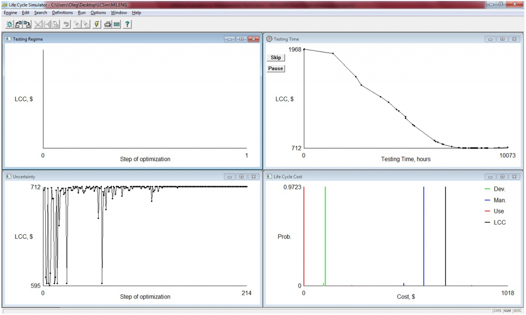
The calculation on the Life Cycle Simulator gives us similar results (Fig. 1)The Life Cycle Simulator is a very complex tool that considers simultaneously up to 12 failure modes with different lifetime distributions (Weibull, lognormal, exponential, etc.) and up to 5 redesign options. The function of the goal can be not only the life cycle cost expectation, but also cost with a given confidence level (for example CL=0,9 or 0,95). We can search for the best acceleration test modes and found completely new accelerated test methods to meet the Time to Market. There is a video of how the Life Cycle Simulator works on YouTube (https://www.youtube.com/watch?v=0_RtgmAzATg&t=68s).

good
Thank you