The term Bayesian Reliability Analysis is popping up more and more frequently in the reliability and risk world. Most veteran reliability engineers just roll their eyes at the term. Most new reliability engineers dread the thought of having to learn something else new, just when they are getting settled in the job. Regardless, it is a really good idea for all reliability engineers to have a basic understanding of Bayesian Reliability Analysis.
This series explains Bayesian Reliability Analysis and justifies reliability engineers at least being familiar with the term. With Bayesian Reliability Analysis, MTBF is at best a useless aside, so this series is a propos for the NoMTBF website.
(Editors note: This was originally published as a five part series. It is combined together in this version.)
Part 1 of 5
I will be using a bit of math (but then, how can you do anything in reliability without math?), but don’t despair, you will discover late in the series that you won’t actually have to do any of the integrals that I will be deriving to practice Bayesian Reliability Analysis.
Let’s suppose that you have a product, and that you are going to make a large number of them. Suppose you have a set of these products that have failed (and the times of service at which they failed – your failure data), and a set of these that have not failed (and their durations of service – your survivor or suspension data).
What you would like to know is the exact reliability of the product. With the exact reliability, you can effectively predict and plan for preventative maintenance, plan and budget for warranty service, and set a competitive price for the product accordingly, among many other things. The reliability can be calculated using a simple integral of the product’s failure probability density function.

Unfortunately, it is impossible to actually know the product’s failure probability distribution, or its density function pd(tf). This means that we will always be uncertain about the reliability,
R(T). This uncertainty about the reliability suggests that there should be a probability distribution model for the reliability, pd(R(T)).
If we could develop that uncertainty distribution model for the reliability, pd(R(T)), then we could calculate the risk that the product’s reliability does not meet or exceed some specified critical reliability value, Rc(T). This could tell us how much risk you might be taking when using a particular preventative maintenance scheme, or risk for warranty costs, or risk in setting the product price, and make some really good decisions.
As a probability statement, this risk looks like this:

The trick of course is to find a way to derive that probability distribution model for the reliability, pd(R(T)), so you can calculate the risk. Next time, we will get started on the derivation for this model.
But We Need our Reliability Distribution Model Based on the Data
Part 2 of 5 of What’s All the Fuss about Bayesian Reliability Analysis?
In part 1, we determined that we are uncertain about the product’s failure model, pd(tf), so we are thus uncertain about the product’s reliability, R(T). If we can calculate the risk that the reliability does not meet some specified critical value, Rc(T), then you can make a lot of really good decisions about maintenance, warranties, pricing etc.. Calculating this risk requires that we integrate the uncertainty model for the reliability, pd(R(T)). But how do we obtain this uncertainty model?
Recall that we do have failure and survivor data. This data, along with the best engineering judgment of the engineers who designed our product, comprise just about all of the information we have related to the product’s failure model, and hence related to the reliability. Design engineers tend in general to look favorably on the products they design, and thus might be a shade optimistic about the reliability of the product they designed. Your failure and survivor data however are completely objective; they happened despite anyone’s opinions on the product.
Any uncertainty distribution models for the product’s failure and reliability are going to have to be based on our failure and survivor data; that is the only objective information we have. Basing these uncertainty models on the data that you have, equations (1) and (2) now look like this:
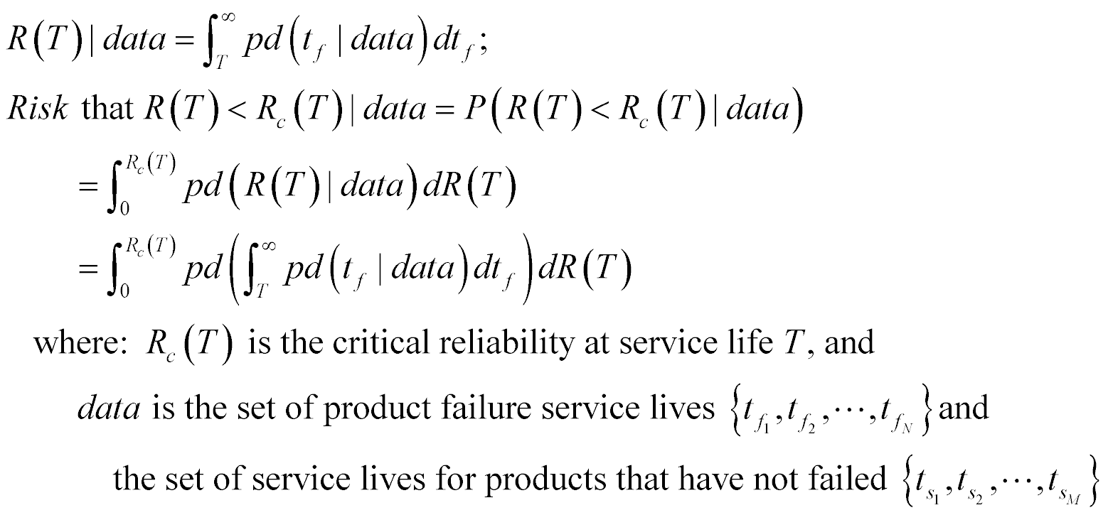
The key still resides with your product’s failure distribution model, which we cannot know exactly. However, we can develop a general form for the product’s failure probability distribution model, pd(tf). We could do this by modeling a thorough engineering analysis of the potential failure modes, or else just use a very general probability distribution model. Presumably, we can validate this form for the model for the product’s failure mode(s).
Whatever approach we use to determine the form of the failure probability distribution model, that model will be based on a set of parameters Θ. The values of the parameters Θ will determine the exact shape of the failure distribution. We write this as pd(tf |Θ).
The uncertainty we have about your product’s failures, assuming that the form of the failure uncertainty model is valid (and with Bayesian Reliability Analysis, we can indeed deal with uncertainty about the form of the model, but that is another series), is now due to uncertainty about the values of those parameters Θ. Based on the form of the failure distribution model,
pd(tf |Θ), we can use your data to develop an uncertainty distribution for the parameters Θ of that model, pd(Θ|data). (Most commercially available reliability tools we use today provide point estimate values (means, or maximum likelihood or mode estimates) for the parameters for a small set of general probability distribution models used for the failure mode, and do not provide the complete joint uncertainty distribution for the parameters. These tools only work with general probability distribution models, and definitely do not work with complex realistic failure models based on engineering analyses.)
But what we actually need to compute our reliability risk is pd(tf|data), not pd(tf |Θ) or
pd(Θ|data). However, if we can develop pd(Θ|data), we can transform pd(tf |Θ) into pd(tf|data) by using pd(Θ|data) as a kernel in an integral transform. Here is that integral transform.

That sounds simple enough. In part 3, we will develop pd(Θ|data) so that we can calculate the reliability risk that we need to make good decisions.
Formulating the Failure Distribution Model based Solely on your Data
Part 3 of 5 of What’s All the Fuss about Bayesian Reliability Analysis?
In part 1, we determined that what we needed in order to make some really important decisions for our product, about things like for maintenance, warranties, pricing, etc., was to know how sure we could be that the reliability of our product meets a specified critical reliability; or in other words, what the risk is that our product doesn’t meet this critical reliability. In our attempt to find out how to calculate this risk in part 2, we ended with the integral transform that would provide your product’s failure probability distribution model based on the failure and survivor data you have, pd(tf|data). Here is how this integral transform factors into our equations (1) and (2) for calculating the risk we need.
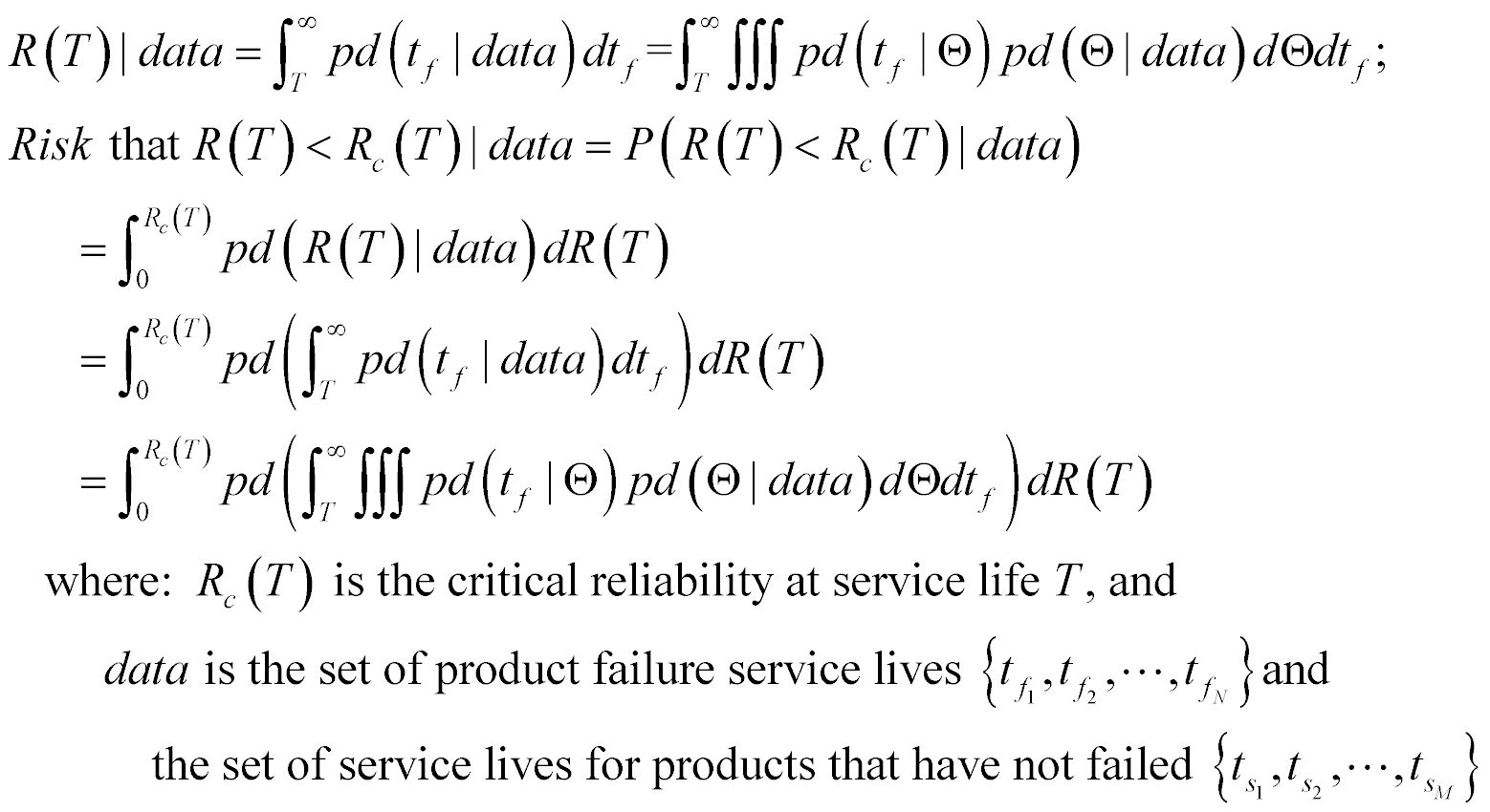
The key now seems to hinge on development of our uncertainty distribution model for the parameters Θ, pd(Θ|data), using the form of the failure distribution model, pd(tf |Θ), based on the data. Using the fourth axiom of probability, and the fact that the Boolean AND operation is commutative, we can write out the following equation for the joint probability for the parameters Θ and the data.

Let’s do some simple algebraic manipulation of the second equality in equation (6).

The proportionality in equation (7) is possible because the probability P(data), the probability of observing the set of data we have, is a simple constant value given the data we have observed.
Our observable universe, and hence the failures of the product about whose reliability we are concerned, can be described as an L2 vector space. In L2 vector spaces, the derivative operator is linear. As a result, the proportion in equation (7) in terms of probabilities can be converted directly into a probability density function equation.

What does equation (8) mean? Well, pd(Θ|data) is the uncertainty model for Θ, the probability density function for Θ given the data. This is of course what we need to solve equation (5).
pd(data|Θ) is the uncertainty model for obtaining our data given values for Θ. If you have used Maximum Likelihood Estimation, you might recognize pd(data|Θ) as the likelihood function. Since our data, both failures and survivors, are independent, this likelihood function is expressible using the form of the failure distribution model, pd(tf|Θ).

pd(Θ), the last term in equation (8), is the marginal uncertainty model for Θ, the probability density for Θ. There is no way to know what this model should be, so the best way to approach this is to be as objective as possible. There are three ways to do this. One is to use the uncertainty model that minimizes the Fisher information in pd(tf|Θ) (developed by Jeffreys in the 1930’s); the second is to use the uncertainty model that maximizes the information entropy in pd(tf|Θ) (entropy is a measure of disorder, so the more information disorder provided by
pd(Θ), the more objective is pd(Θ) – developed by Lindley and Savage in the 1960’s); and, the third is to use the uncertainty model that maximizes the Expected Value of Perfect Information for pd(tf|Θ) (EVPI is a measure of how much the uncertainty can be reduced with perfect information, the larger the EVPI with pd(Θ), the more objective is pd(Θ) – developed by Bernardo and Smith in the 1990’s). Which method should you use to find an objective pd(Θ)? Interestingly enough, for every failure distribution model formulation that I have ever seen, all three methods produce the exact same model for pd(Θ) for that formulation. That is really comforting since the three methods all approach finding the most objective model pd(Θ) from such different perspectives.
Using such an objective model for pd(Θ), we end up with:

When we insert equation (10) into equation (4), we obtain:

In part 4, we will put it all together to enable us to calculate that risk we need to make those important decisions.
Calculating the Risk of not Meeting a Critical Reliability Specification
Part 4 of 5 of What’s All the Fuss about Bayesian Reliability Analysis?
In part 1 of this series, we determined that what we really needed in order to make some really important decisions for our product, about things like maintenance, warranties, pricing, etc., was to know how sure we could be that the reliability of our product meets a specified critical reliability; or in other words, what the risk is that our product doesn’t meet this critical reliability.
In our attempt to find out how to calculate this risk in part 2, we concluded with the integral transform that would provide your product’s failure probability distribution model based on the failure and survivor data you have, pd(tf|data). But that analytical transform was still in terms of the parameters Θ of the form of our product’s failure distribution model, not the data directly.
In part 3, we finally were able to get rid of the parameters Θ altogether, and obtain an analytical expression for your product’s failure probability distribution model pd(tf|data), purely in terms of just the data we have, our failure and survivor data.
Here is how that solution for pd(tf|data) from equation (11), purely in terms of just the data we have, our failures and survivors, factors into our equation (1) for the reliability and equation (2) for the risk that the reliability does not meet our specified critical reliability.
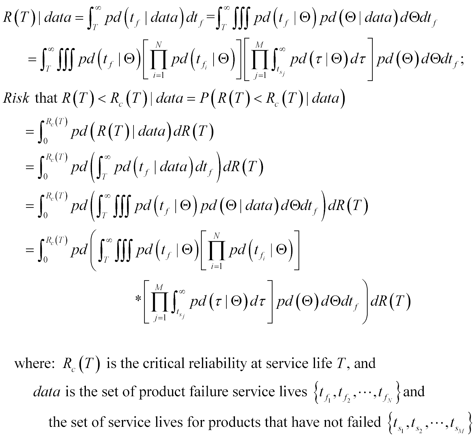
We now have the solution, expressed analytically, for computing the risk of our product’s reliability not meeting or exceeding the specified critical reliability, Rc(T), all based on your data. This process to derive this equation has seemed very complex, but is actually rather straightforward to solve with but three steps. These were to:
1) Formulate a model for your product’s failure distribution model in terms of a set of parameters Θ, pd(tf|Θ). You can base this form for your product’s failure distribution model either on an engineering analysis of the possible failure modes, or use a general failure distribution model. And, don’t forget to validate this form for your product’s failure distribution model.
2) Using that form for your product’s failure distribution model, find an objective uncertainty model for its parameters Θ, pd(Θ), using one of the three methods we discussed in part 3 (conveniently, these objective models for the parameters Θ have already been developed for most general models used for reliability, and are listed in a number of references – you almost never have to do all that math for reliability related problems).
3) Into equations (12), plug in the form for your product’s failure distribution model, pd(tf|Θ), the objective uncertainty model for its parameters Θ, pd(Θ), your failure and survivor data, and solve equation (12).
With that risk value we just computed, based solely on the data without making any questionable assumptions, we can now comfortably make all of those important decisions we need to make about maintenance, warranty, pricing, etc..
Let me provide an example of how this works. Suppose we decided to use the most general unimodal one-sided model available for our product’s failure distribution model, the Weibull model (and validated that it is suitable). It has a scale parameter η and a shape parameter β. The objective uncertainty models for η and β using any of the three methods we discussed in part 3 are simple inverses, so pd(Θ)~(1/η)*(1/β). Here is how equations (12) would be expressed substituting the form of the Weibull model and these objective uncertainty models.
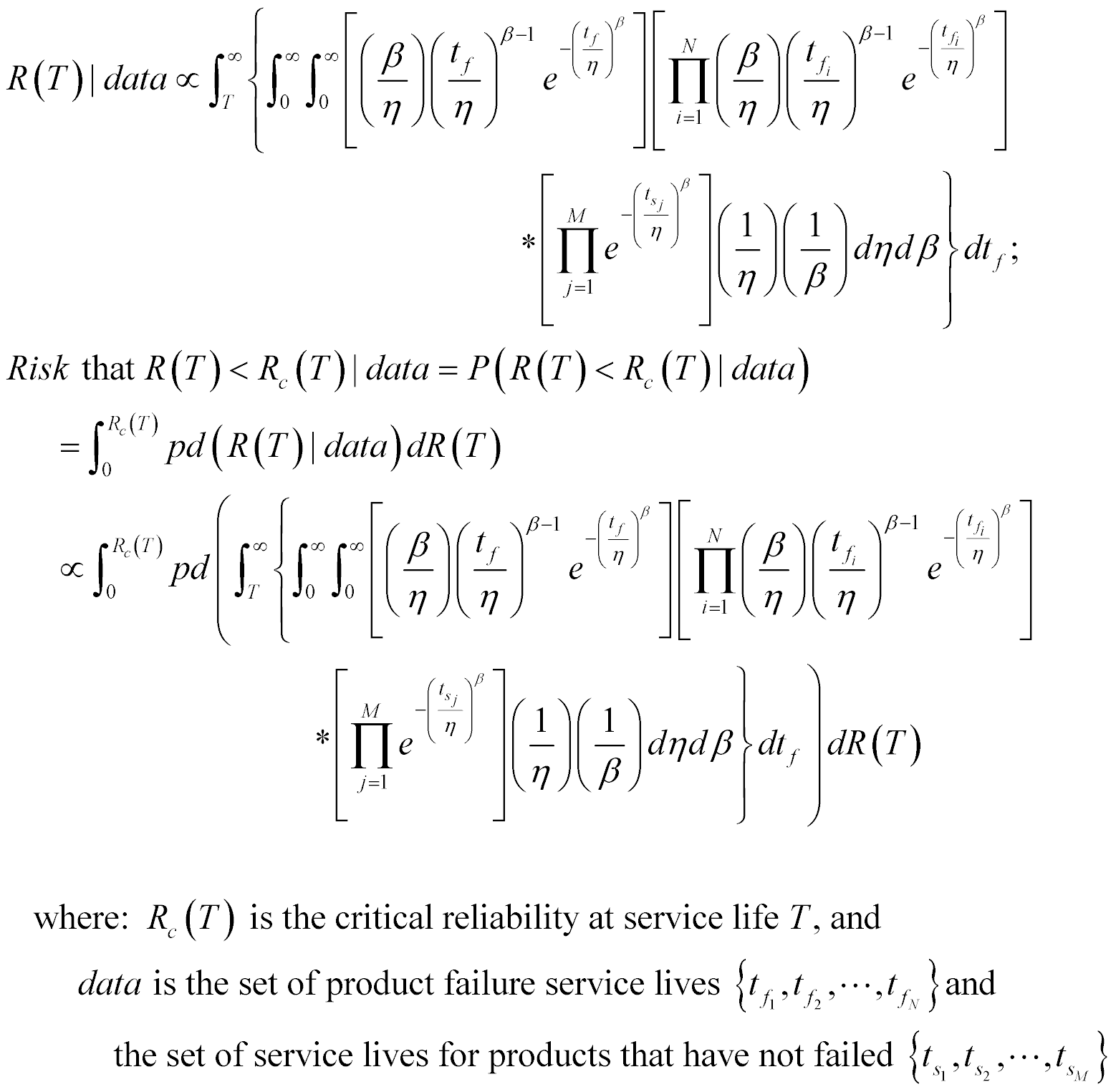
Equations (12) and (13) look daunting don’t they. They are daunting! Equations (12) is almost always impossible to solve analytically for real world reliability problems (I have never seen a case where it could be, not even a textbook example). Equations (13) are clearly not solvable analytically.
So, to obtain any sort of solution, we have to resort to numerical methods. Amazingly, numerical methods make the solution for equations (12) almost too easy to believe.
The numerical method we will use is Monte Carlo (MC). The Monte Carlo method is used to obtain approximate solutions for definite integrals. The last (and outermost) integral in equations (12) is a definite integral. MC methods also can be used to perform integral transformations, such as the inner-most integral transform in equations (12) or in equation (4).
The Monte Carlo method requires that we first obtain samples of the parameters Θ from the uncertainty distribution for Θ in equation (10). Sampling algorithms for the multivariate joint probability distribution model in equation (10) do not exist built-in in any reliability tools. So we have to resort to Markov Chain Monte Carlo (MCMC) methods. The difference between MCMC and ordinary MC is that MCMC uses a Markov chain to generate joint random samples of the integrand whereas ordinary MC uses built-in random sampling algorithms (but only for integrands recognizable as one of the common probability distribution models, e.g., Gaussian, uniform, gamma, etc.). Using MCMC, we can sample very high dimension multivariate joint probability distributions (up to 20,000 correlated random variables in the literature) and compute all sorts of marginal and conditional probability integrals from the samples of the joint distributions.
We will want to obtain a large number of joint samples of the parameters Θ to assure that we get good coverage of the whole joint distribution, say no fewer than 10,000 sets. Larger numbers of samples also reduces the numerical method error as well.
Now, for almost all reliability problems that we will encounter, the form we use for the product’s failure probability distribution, pd(tf|Θ), will result in equation (1) having a nice closed form analytical solution in terms of the parameters Θ. Thus, we have:

For the example we used to form equations (13), based on using the Weibull model as a form for our product’s failure distribution model, pd(tf|Θ), we do obtain a rather nice closed form analytical solution.
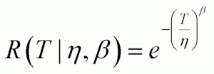
If we evaluate R(T|Θ) in equation (14) at each of the joint MCMC samples of the parameters Θ, we will produce samples of R(T)|data from that complex multi-integral density function
pd(R(T)|data) that appears in equations (12). This seems almost magical, but it works (and can be proven mathematically, but that would be an even longer series).
For our example using the Weibull model, equation (10) that provides the uncertainty model for the parameters for the form of our product’s failure distribution model, based solely on the data, looks like the following.

Clearly, there is no random sampler for η and β using equation (16) built-in in any reliability tool. So, we use MCMC to obtain joint samples of η and β using equation (16), and substitute these joint samples (η, βi) into equation (15). We thus obtain samples of Ri(T|η, β) based solely on the data we have, our failures and survivors.

Now all we have to do to calculate an approximate value for the risk we need to make good decisions is to count the number of the samples of Ri(T)|data that are less than the critical reliability Rc(T), and divide by the total number of samples.
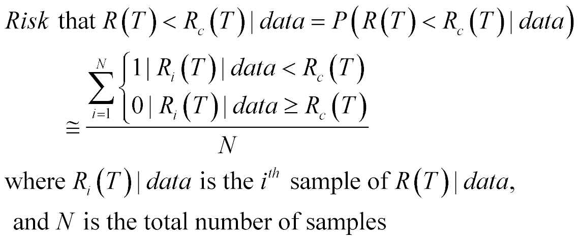
Wowee! Does that ever simplify things! No assumptions; our solution for our reliability risk is based purely on the objective data. Those decisions become ever so much easier and comfortable.
Equation (18), after obtaining our joint samples of the parameters Θ using equation (10) and evaluating them using equation (14), gives us an approximate value for the risk of our product’s reliability not meeting or exceeding our critical reliability, Rc(T), based solely on the data. If we generated enough joint samples of the parameters Θ, the error in this approximation of risk can be quite small, down to the third or fourth significant digit, far too small to interfere with good decision making. (Should you not be able to find a nice closed form analytical solution for your product’s reliability in terms of the parameters Θ as in equation (14), there are a few additional steps needed to use these samples to solve the more general problem, but it is still very easy to do. Contact me (mark.powell@AttwaterConsulting.com) if you run into this problem and need those steps and I can show you how to do it.)
Note that we did not say a single word about Bayesian Reliability Analysis in this entire derivation and solution of our problem in parts 1-4 of this series. Why the title of this series then? We will conclude in part 5 with the answer.
So, What is All the Fuss about Bayesian Reliability Analysis?
Part 5 of 5 of What’s All the Fuss about Bayesian Reliability Analysis?
In parts 1, 2, 3, and 4, we derived an analytical equation for how sure we can be that the reliability of our product meets a specified critical reliability, based solely on our failure and survivor data. In other words, we developed an analytical equation for the risk that our product doesn’t meet this critical reliability, in terms of just our failure and survivor data. This risk is the primary factor that enables us to make a lot of really important decisions about our product, things like maintenance schedules, warranty policies, pricing, etc. We then showed that we could obtain an approximate quantitative numerical solution for this risk that could be more than accurate enough to make good decisions. Conveniently, in this entire process we did not have to resort to making any questionable assumptions about anything; we started with first principles, and abided by all the rules of mathematics and the axioms of probability; no tricks, just straightforward albeit busy and sometimes what seemed like complex math.
The topic of this series however is Bayesian Reliability Analysis. Here is the connection.
You may have never seen the analytical derivation of equation (12) that we developed in this series. You probably cannot find it in any textbook or documentation for any reliability tool either. This makes a lot of sense actually. It is not possible to solve equation (12) analytically, so why teach it? It is not possible to solve it using ordinary numerical methods, including ordinary Monte Carlo methods that can be implemented in a general reliability tool, so why teach it or include it in any reliability tool documentation?
In part 4, we showed how to obtain an approximate numerical solution to this problem using Markov Chain Monte Carlo (MCMC) methods. MCMC methods only began to appear in the literature in the mid 1990’s, and they were applied to biostatistics risk problems in European medical journals. Unfortunately, except for some very special problems (the set of which does not include reliability problems where you avoid a bunch of questionable assumptions), MCMC methods cannot be implemented in a general reliability tool; they have to be coded up specifically for every problem. Fortunately, MCMC methods are really simple to code, and don’t take much code at all. Because of this inability to develop a general tool using MCMC for reliability problems, it is no surprise that reliability tool vendors don’t bother including a derivation of equation (12) in their documentation.
Instead, methods from classical statistics have been taught and used for reliability analysis for more than 80 years, and built into commercially available reliability tools. These methods produce point estimates for the parameter values (including moments such as MTBF) for a limited set of failure distribution models (not models derived from engineering analyses of the failure modes). These classically derived point estimates can then be plugged into reliability and risk equations as if they are the true values (clearly, they are not, they are just estimates). Quite often, the results from plugging these point estimates into reliability and risk equations do not make decision making for many important product and business decisions very comfortable. The assumptions required to develop these point estimates make many decision makers very wary of the results. Many, many discussions on LinkedIn reliability groups exhibit this discomfort, but in most cases the discussion participants cannot pinpoint exactly why they are uncomfortable. Of course, a thorough analysis of the assumptions necessary to compute these point estimates should make everyone uncomfortable making decisions using their plug-in-the-point-estimates results, but that is another topic altogether.
To distinguish what we developed analytically in parts 1-4 of this series from the classical methods you have been taught, and that are implemented in commercially available reliability tools, a lot of folks are now referring to what I presented in parts 1-4 as Bayesian Reliability Analysis. Why, you might ask?
Well, Equations (7) in part 3 is the derivation of Bayes’ law. The derivation of Bayes’ law is just that simple; a two line scalar division applied to the fourth axiom of probability. It played but a minor but necessary role in our analytical derivation of equation (12). Yet, because Bayes’ law is used, folks have started calling what we did in parts 1-4 Bayesian Reliability Analysis, introducing a new buzzword.
Me, I think what we did in parts 1-4 should be called The Only Way to do Reliability Analysis, but that does not sound very good as a buzzword. After all, we started with first principles, derived our equations correctly in accordance with all the rules of mathematics and the axioms of probability, did not employ any questionable assumptions, and produced the ability to provide risk answers based solely on the data. This allows a lot of important decision making, without a lot of discomfort for the decision makers.
Hopefully, the readers who have made it this far appreciate the analytical derivations and solutions via numerical methods in parts 1-4. We actually went through some fairly complex math. And the fact that we can indeed obtain useful numerical solutions as simply as we did is almost magical. The very understanding alone that we can indeed analytically formulate the equations in parts 1-4 should provide some very useful insights for all of your reliability analyses. Plus, you can now solve a lot of rather complex reliability related problems, and make a lot of good decisions rather cleanly and comfortably, that perhaps classical statistical approaches have left less clean and comforting.
If you would like to see some examples of the types of rather complex reliability related problems and decisions that have actually been made quickly and comfortably using Bayesian Reliability Analysis, you can find a few of the papers that I have published solving these problems at:
http://www.attwaterconsulting.com/Papers.htm.
If you would like copies of the papers or wish to contact me about this series, my e-mail address is Mark.Powell@AttwaterConsulting.com.
So, what is all the fuss about Bayesian Reliability Analysis? Maybe it is that we can finally do reliability right.